GPS 103: GMM Activity Classification and Validation
Source:vignettes/gps-103-activity-and-validation.Rmd
gps-103-activity-and-validation.RmdOverview
This tutorial covers the next stage after cleaning and metric generation:
- classify each GPS row as
activeorinactivewith GMM, - smooth state flicker with HMM-based temporal smoothing,
- manually label rows in an interactive app,
- compare model predictions against labels,
- rank parameter settings by agreement.
Why This Workflow?
State classification is iterative. A clear validation loop gives better decisions:
- You can inspect how model assumptions map to real movement behaviour.
- You can use manual labels as a transparent ground-truth reference.
- You can tune parameters with a reproducible and auditable process.
- You can report uncertainty and model agreement directly.
2) Build a small reproducible example
set.seed(202)

timestamps <- seq(
  from = as.POSIXct("2024-06-01 00:00:00", tz = "UTC"),
  by = "10 min",
  length.out = 3 * 24 * 6
)

animal_info <- tibble(
  sensor_id = c("A01", "A02"),
  lon0 = c(132.310, 132.316),
  lat0 = c(-14.462, -14.467)
)

gps_list <- list()
for (i in seq_len(nrow(animal_info))) {
  gps_list[[i]] <- tibble(
    sensor_id = animal_info$sensor_id[i],
    datetime = timestamps,
    lon = animal_info$lon0[i] + cumsum(rnorm(length(timestamps), 0, 0.00020)),
    lat = animal_info$lat0[i] + cumsum(rnorm(length(timestamps), 0, 0.00016))
  )
}
gps <- bind_rows(gps_list)

gps <- grz_clean(
  data = gps,
  steps = c("errors", "speed_fixed", "denoise"),
  max_speed_mps = 4,
  verbose = FALSE
)
How this works in practice:
- Start from already cleaned GPS rows with stable identifiers.
- Keep example windows small enough to iterate quickly while tuning.
Common pitfalls and checks:
- Pitfall: tuning on too broad a window early on.
Check: begin with one animal and a short period, then scale up.
3) Run GMM active/inactive classification
grz_classify_activity_gmm() fits a two-component
Gaussian mixture on movement features, then can apply optional HMM
smoothing to reduce rapid state flicker.
gps_states <- grz_classify_activity_gmm(
  data = gps,
  groups = "sensor_id",
  feature_set = "adaptive",
  adaptive_window_mins = "auto",
  adaptive_window_mult = 4,
  adaptive_window_min_mins = 30,
  smoothing = "hmm",
  hmm_self_transition = 0.98,
  verbose = FALSE
)

state_view <- gps_states %>%
  as_tibble() %>%
  select(sensor_id, datetime, lon, lat, activity_state_gmm, inactive_prob_gmm)

state_view
#> # A tibble: 864 × 6
#>    sensor_id datetime              lon   lat activity_state_gmm
#>    <chr>     <dttm>              <dbl> <dbl> <chr>
#>  1 A01       2024-06-01 00:00:00  132. -14.5 NA
#>  2 A01       2024-06-01 00:10:00  132. -14.5 NA
#>  3 A01       2024-06-01 00:20:00  132. -14.5 active
#>  4 A01       2024-06-01 00:30:00  132. -14.5 active
#>  5 A01       2024-06-01 00:40:00  132. -14.5 active
#>  6 A01       2024-06-01 00:50:00  132. -14.5 active
#>  7 A01       2024-06-01 01:00:00  132. -14.5 active
#>  8 A01       2024-06-01 01:10:00  132. -14.5 active
#>  9 A01       2024-06-01 01:20:00  132. -14.5 active
#> 10 A01       2024-06-01 01:30:00  132. -14.5 inactive
#> # ℹ 854 more rows
#> # ℹ 1 more variable: inactive_prob_gmm <dbl>

state_more <- setdiff(names(gps_states), names(state_view))
cat(
  "i",
  length(state_more),
  "more columns:",
  paste(head(state_more, 10), collapse = ", "),
  if (length(state_more) > 10) ", ..." else "",
  "\n"
)
#> i 10 more columns: lon_raw, lat_raw, step_dt_s, step_m, speed_mps, bearing_deg, turn_rad, cum_distance_m, net_displacement_m, activity_component_gmm
Key state variables in this workflow:
-
activity_state_gmm: finalactive/inactivestate after optional smoothing. -
inactive_prob_gmm: inactivity probability (smoothed ifsmoothing = "hmm"). -
activity_component_gmm: assigned mixture component id.
How this works in practice:
- GMM separates low-movement and high-movement behaviour from engineered features.
- Optional HMM smoothing adds temporal consistency to state sequences.
Common pitfalls and checks:
- Pitfall: assuming one setting is always correct across
deployments.
Check: tune and validate on representative subsets. - Pitfall: class imbalance leading to misleading accuracy.
Check: inspect class proportions by day and animal.
gps_states %>%
  as_tibble() %>%
  ggplot(aes(x = lon, y = lat, color = activity_state_gmm)) +
  geom_point(alpha = 0.7, size = 1.3) +
  facet_wrap(~sensor_id, scales = "free") +
  scale_color_manual(values = c(active = "#1a9641", inactive = "#d7191c")) +
  labs(
    title = "GMM Activity State Classification in Space",
    x = "Longitude",
    y = "Latitude",
    color = "State"
  ) +
  theme_minimal()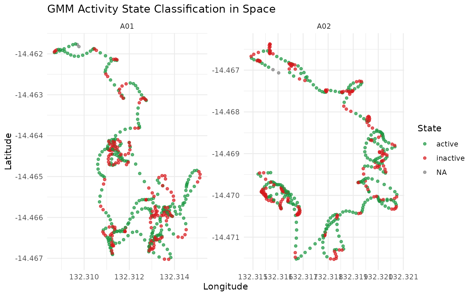
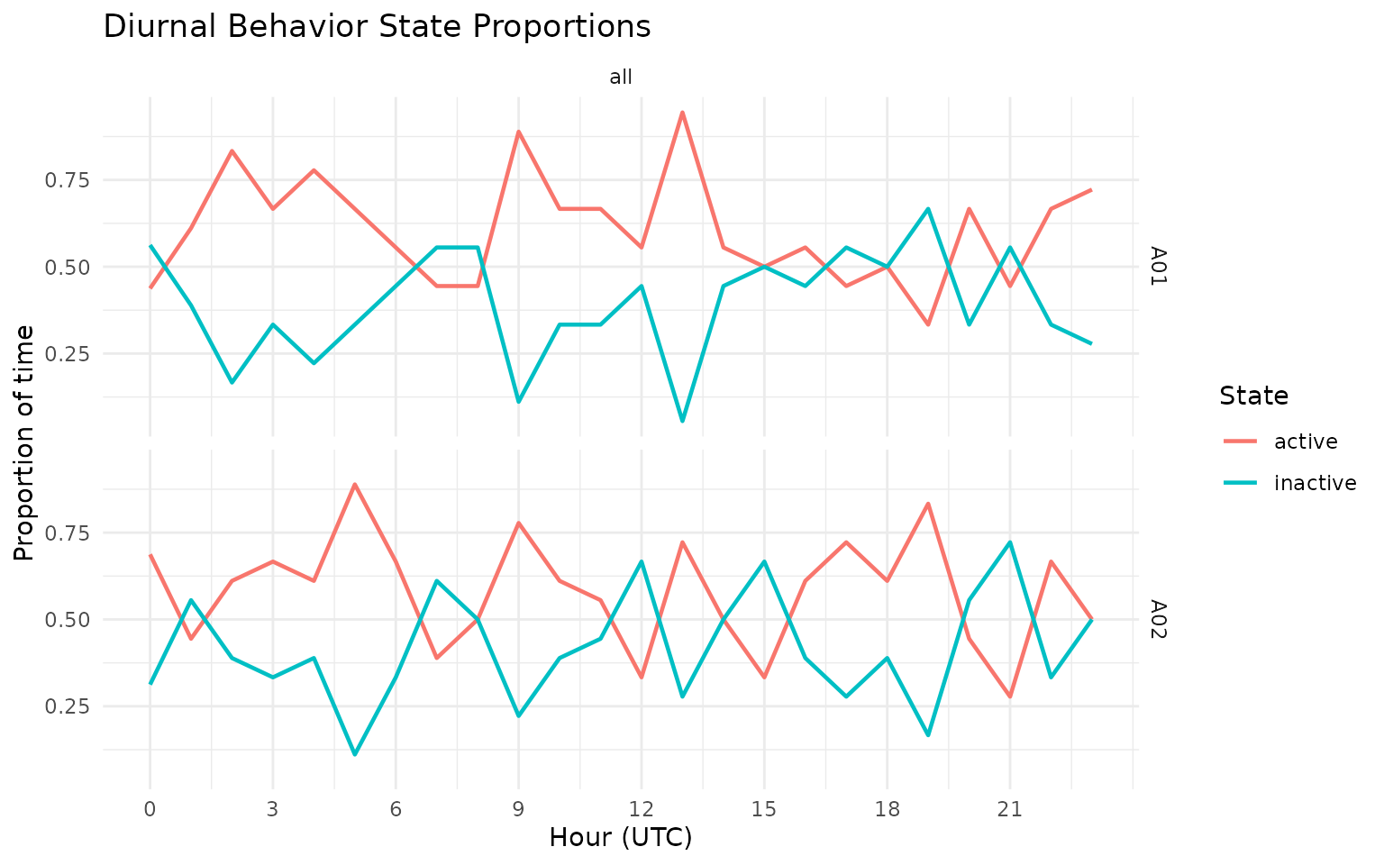
grz_plot_diurnal_states(
  data = gps_states,
  state_col = "activity_state_gmm",
  group_col = "sensor_id",
  plot_type = "line"
)
gps_states %>%
  as_tibble() %>%
  mutate(day = as.Date(datetime)) %>%
  group_by(sensor_id, day, activity_state_gmm) %>%
  summarise(n = n(), .groups = "drop") %>%
  group_by(sensor_id, day) %>%
  mutate(prop = n / sum(n)) %>%
  ungroup() %>%
  ggplot(aes(x = day, y = prop, fill = activity_state_gmm)) +
  geom_col(position = "stack") +
  facet_wrap(~sensor_id) +
  scale_fill_manual(values = c(active = "#1a9641", inactive = "#d7191c")) +
  labs(
    title = "Daily Proportion of Active vs Inactive States",
    x = "Day",
    y = "Proportion of fixes",
    fill = "State"
  ) +
  theme_minimal()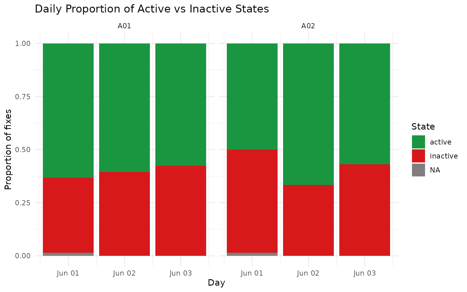
4) Add manual labels (interactive app)
Use this in an interactive R session to create or edit a
label column.
gps_states$point_id <- paste(
  gps_states$sensor_id,
  format(gps_states$datetime, "%Y%m%d%H%M%S", tz = "UTC"),
  seq_len(nrow(gps_states)),
  sep = "_"
)

labelled <- grz_label_gps_states(
  data = gps_states,
  lon = "lon",
  lat = "lat",
  time = "datetime",
  id = "point_id",
  color_by = "sensor_id",
  initial_label_col = "label",
  start_day_offset = 0L,
  time_window = "week",
  n_animals = 1L,
  animal_col = "sensor_id"
)
If you save that output to CSV, you can reload it later and continue editing:
# data.table::fwrite(labelled, "labelled_states.csv")
# labelled <- data.table::fread("labelled_states.csv")
# labelled$datetime <- as.POSIXct(labelled$datetime, tz = "UTC")
How this works in practice:
- Manual labels provide ground truth for calibration and validation.
- Labels should be saved with stable IDs so they can be reused across sessions.
Common pitfalls and checks:
- Pitfall: relabelling the same points without versioning.
Check: keep dated label files or append a reviewer/version column. - Pitfall: using ambiguous behaviour windows.
Check: mark uncertain points asNAinstead of forcing a label.
5) Demonstrate a prediction-vs-label comparison
For a fully reproducible vignette, we create a synthetic
label column by copying predictions and flipping a random
subset of rows.
In your project, replace this with manual labels from
grz_label_gps_states().
labelled <- gps_states
labelled$label <- labelled$activity_state_gmm

set.seed(303)
flip_n <- floor(0.1 * nrow(labelled))
flip_idx <- sample(seq_len(nrow(labelled)), size = flip_n)

labelled$label[flip_idx] <- ifelse(
  labelled$label[flip_idx] == "active",
  "inactive",
  "active"
)

label_view <- labelled %>%
  as_tibble() %>%
  select(sensor_id, datetime, activity_state_gmm, label, inactive_prob_gmm)

label_view
#> # A tibble: 864 × 5
#>    sensor_id datetime            activity_state_gmm label    inactive_prob_gmm
#>    <chr>     <dttm>              <chr>              <chr>                <dbl>
#>  1 A01       2024-06-01 00:00:00 NA                 NA            NA
#>  2 A01       2024-06-01 00:10:00 NA                 NA            NA
#>  3 A01       2024-06-01 00:20:00 active             active         0.000999
#>  4 A01       2024-06-01 00:30:00 active             active         0.000256
#>  5 A01       2024-06-01 00:40:00 active             inactive       0.000000155
#>  6 A01       2024-06-01 00:50:00 active             active         0.000000120
#>  7 A01       2024-06-01 01:00:00 active             active         0.000000132
#>  8 A01       2024-06-01 01:10:00 active             active         0.000000322
#>  9 A01       2024-06-01 01:20:00 active             active         0.000708
#> 10 A01       2024-06-01 01:30:00 inactive           inactive       1.000
#> # ℹ 854 more rows

label_more <- setdiff(names(labelled), names(label_view))
cat(
  "i",
  length(label_more),
  "more columns:",
  paste(head(label_more, 10), collapse = ", "),
  if (length(label_more) > 10) ", ..." else "",
  "\n"
)
#> i 12 more columns: lon, lat, lon_raw, lat_raw, step_dt_s, step_m, speed_mps, bearing_deg, turn_rad, cum_distance_m , ...
How this works in practice:
- Truth labels and predicted states are compared on the same rows.
- Only valid binary states (
active,inactive) are included for scoring.
6) Tune parameters and rank the top 3 settings
grid <- tidyr::expand_grid(
  adaptive_window_mult = c(3, 4, 5),
  hmm_self_transition = c(0.95, 0.975, 0.99)
)

results <- tibble()

for (i in seq_len(nrow(grid))) {
  pred <- grz_classify_activity_gmm(
    data = labelled,
    groups = "sensor_id",
    feature_set = "adaptive",
    adaptive_window_mins = "auto",
    adaptive_window_mult = grid$adaptive_window_mult[[i]],
    adaptive_window_min_mins = 30,
    smoothing = "hmm",
    hmm_self_transition = grid$hmm_self_transition[[i]],
    verbose = FALSE
  )

  comparison <- tibble(
    truth = tolower(trimws(as.character(labelled$label))),
    pred = tolower(trimws(as.character(pred$activity_state_gmm)))
  ) %>%
    filter(truth %in% c("active", "inactive")) %>%
    filter(pred %in% c("active", "inactive"))

  n_compared <- nrow(comparison)
  accuracy <- if (n_compared == 0L) {
    NA_real_
  } else {
    mean(comparison$truth == comparison$pred)
  }

  results <- bind_rows(
    results,
    tibble(
      adaptive_window_mult = grid$adaptive_window_mult[[i]],
      hmm_self_transition = grid$hmm_self_transition[[i]],
      n_compared = n_compared,
      accuracy = accuracy
    )
  )
}

top3 <- results %>%
  arrange(desc(accuracy), desc(n_compared)) %>%
  slice_head(n = 3) %>%
  mutate(accuracy_percent = round(100 * accuracy, 2)) %>%
  select(adaptive_window_mult, hmm_self_transition, n_compared, accuracy_percent)

top3
#> # A tibble: 3 × 4
#>   adaptive_window_mult hmm_self_transition n_compared accuracy_percent
#>                  <dbl>               <dbl>      <int>            <dbl>
#> 1                    4               0.975        860             90.1
#> 2                    4               0.99         860             89.5
#> 3                    4               0.95         860             88.7
How this works in practice:
- A parameter grid is evaluated with a consistent GMM+HMM configuration.
- Each setting is ranked by observed agreement against manual labels.
- Top settings are candidates for holdout validation, not automatic final choices.
results %>%
  mutate(accuracy_percent = 100 * accuracy) %>%
  ggplot(aes(x = factor(adaptive_window_mult), y = factor(hmm_self_transition), fill = accuracy_percent)) +
  geom_tile(color = "white") +
  labs(
    title = "GMM Accuracy Across Parameter Grid",
    x = "adaptive_window_mult",
    y = "hmm_self_transition",
    fill = "Accuracy (%)"
  ) +
  theme_minimal()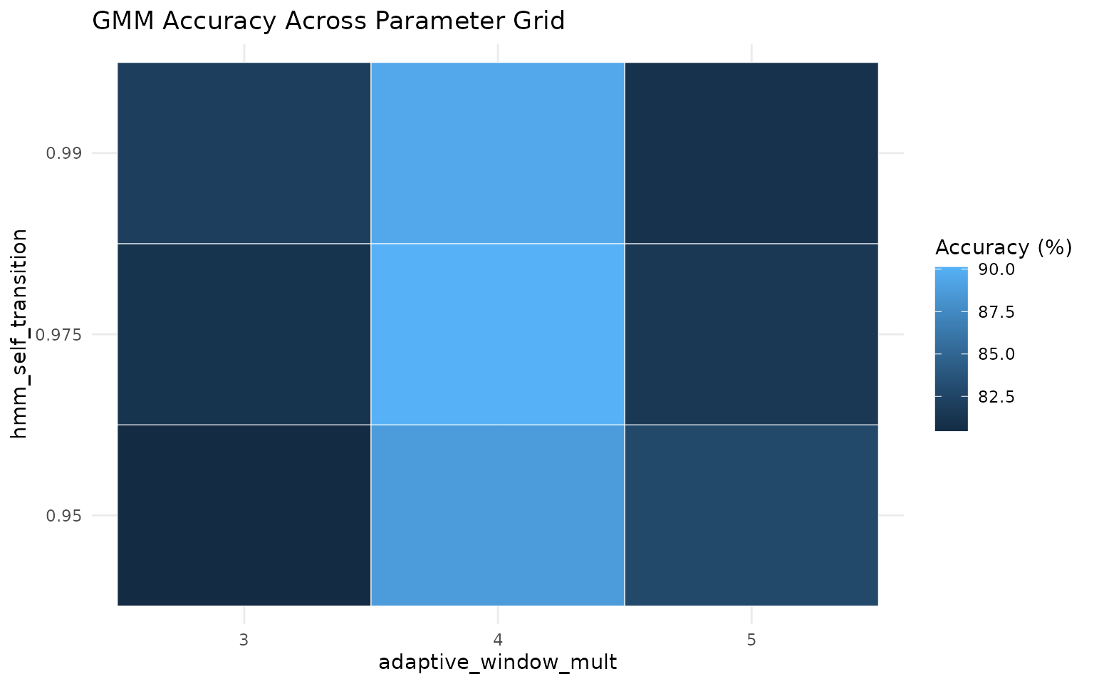
best <- top3 %>% slice(1)

best_pred <- grz_classify_activity_gmm(
  data = labelled,
  groups = "sensor_id",
  feature_set = "adaptive",
  adaptive_window_mins = "auto",
  adaptive_window_mult = best$adaptive_window_mult[[1]],
  adaptive_window_min_mins = 30,
  smoothing = "hmm",
  hmm_self_transition = best$hmm_self_transition[[1]],
  verbose = FALSE
)

confusion_df <- tibble(
  truth = tolower(trimws(as.character(labelled$label))),
  pred = tolower(trimws(as.character(best_pred$activity_state_gmm)))
) %>%
  filter(truth %in% c("active", "inactive")) %>%
  filter(pred %in% c("active", "inactive")) %>%
  count(truth, pred, .drop = FALSE)

confusion_df %>%
  ggplot(aes(x = truth, y = pred, fill = n)) +
  geom_tile(color = "white") +
  geom_text(aes(label = n), size = 5) +
  labs(
    title = "Confusion Matrix for Best Parameter Set",
    x = "Manual label",
    y = "Predicted state",
    fill = "Count"
  ) +
  theme_minimal()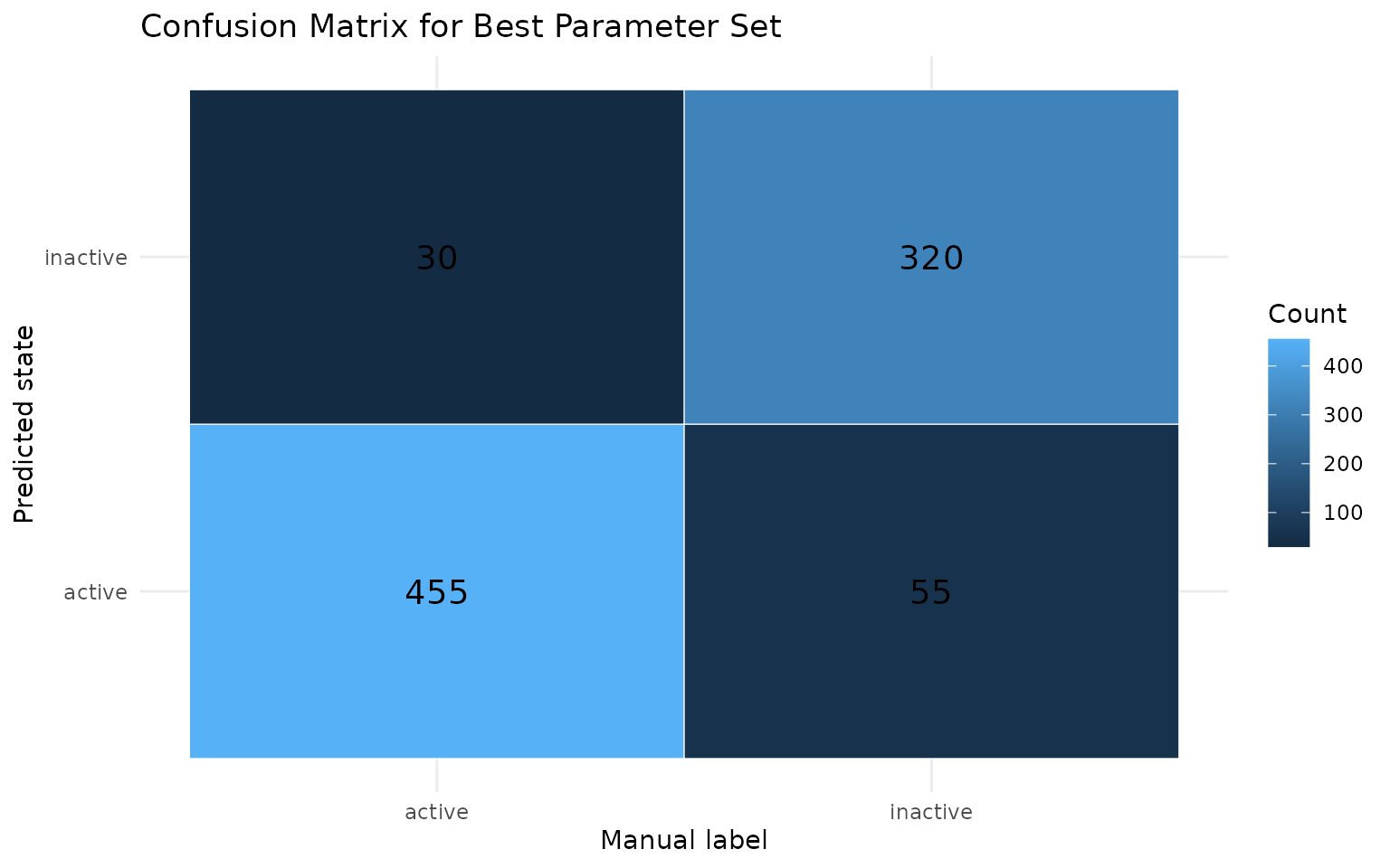
7) Optional advanced diagnostics
These helpers are useful once you have enough labelled data:
# Diurnal feature patterns for threshold setting
grz_plot_diurnal_metrics(
  data = labelled,
  metrics = c("step_m", "turn_rad"),
  group_col = "sensor_id"
)

# Behaviour diagnostics (feature summary, transitions, bouts, PCA)
diagnostics <- grz_validate_behavior(
  data = labelled,
  state_col = "activity_state_gmm",
  groups = "sensor_id",
  pca = TRUE
)
grz_validate_behavior() returns state counts,
transitions, bout summaries, and an optional PCA diagnostic for the
selected state column.